OeS 6 software is intended for modeling and calculation of radial and multiply closed power networks, under operating and short-circuit conditions. The program’s computational capabilities allow for the analysis of the operation of HV, MV and LV networks within one model. The program is also equipped with modules supporting the selection of protection settings and determining the load capacity of cables depending on the installation conditions. OeS has always been created as an engineering tool – it is characterized by transparency and simplicity of use, while maintaining a full range of computational functionalities for the implementation of analytical and design tasks.

Individual OeS software modules allow you to perform power flow and short-circuit calculations, which are an indispensable element of every project or connection expertise. Available functionalities enable, among others: proper selection of devices with regard to operation in operating and short-circuit conditions, solving problems related to reactive power compensation or assessment of the operation of the neutral point. They also support planning the expansion of the existing network and help in making connection decisions. In the OeS software, you can quickly perform calculations for any network configuration, which opens up great opportunities for users to create multi-variant analyses.

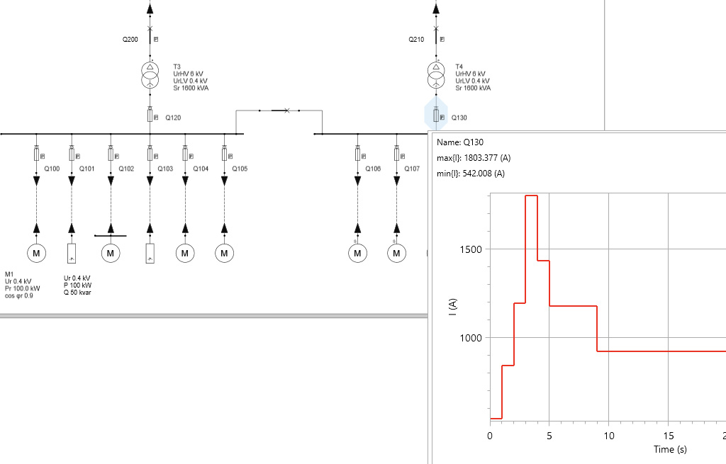
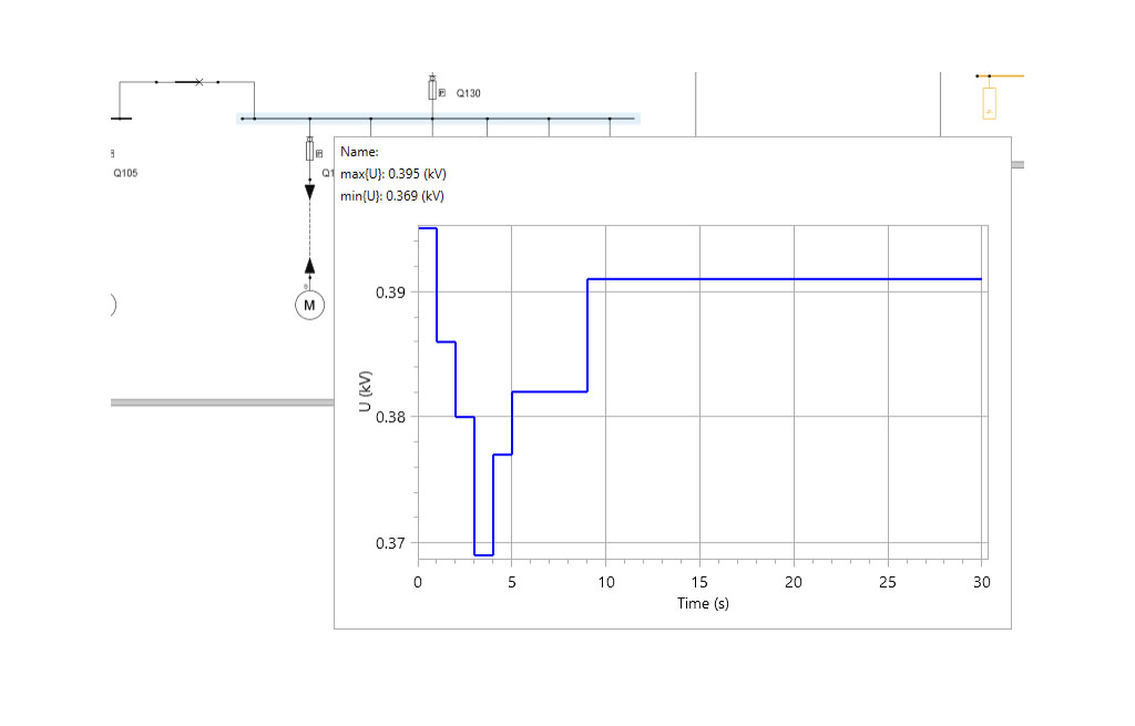
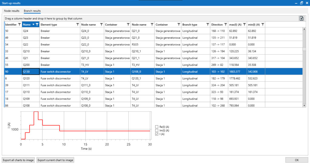
Functionalities related to modeling and analysis of network security operation have also been developed for many years. The user can analyze the sensitivity and selectivity of protections, determine their response times, and assess the risk of shock. Additionally, OeS can be equipped with the PROKAB module, which allows for the creation and calculation of the longitudinal and transverse profiles of the cable and the determination of substitute parameters for overhead lines. Another additional element is the GRAFIK module, which allows for the modeling of consumers taking into account the variability of the load over time (operator’s tariff or measurement data) and the modeling of prosumers taking into account the variability of their generation. The possibility of using the ENTSO-E database (climate years) has been implemented here, taking into account the weather forecast in the calculations or entering measurement data. Computational functionalities allow for the analysis of time histories of power and branch currents, voltages in network nodes, losses and other network parameters.

Motor start

The module is used to perform calculations in the starting conditions of rotating machines. After specifying the starting times and starting moments of individual machines, it is possible to determine the approximate time course of currents and voltages in the network. The module enables analysis of many machines at the same time during startup. The calculation results also include the steady state before and after the start-up sequence.

Start-up calculations allow you to determine the network condition when rotating machines are turned on. The start-up is modeled using a load jump, up to a value resulting from the multiplicity of the starting current (technical parameter of the machines). After the start-up process is completed, the generated load returns to the operating level resulting from the total load factor.

The parameters necessary for machine start-up calculations that must be provided in their dialog windows are:

  • start-up power factor cosϕLR – power factor taken into account during start-up, in the absence of data it is recommended to adopt the value cosϕLR = 0.3,
  • turn-on moment tstart(s) – time moment from which the start-up will be simulated; it is assumed that the machine is not working in the time preceding the moment of switching on,
  • start-up time tr(s) – boot duration starting from tstart; after the start-up is completed, the machine load returns to the operating current level,
  • times the starting current ILR/Ir.

The basic result of the start-up calculations are the time histories of the instantaneous values of currents and voltages for the total analysis time. These waveforms – designated for all branches and nodes of the diagram – are available after moving the mouse cursor over any branch (current waveform) or node (voltage waveform) of the diagram. Full results of the startup calculations are available in the result window:

  • Node Results tab:
    • maximum voltage max{|U|} (kV) – maximum value of the voltage module in the analyzed interval,
    • minimum voltage min{|U|} (kV) – minimum value of the voltage module in the analyzed interval,
    • actual voltage Up(kV) – nodal voltage resulting from the actual transformer ratio,
    • voltage modulus |Uts|(kV) – voltage modulus at the node for the calculation interval starting at time t (s),
    • real part of voltage Re{Uts} (kV),
    • imaginary part of voltage Im{Uts} (kV),
  • Branch Results tab:
    • maximum current max{|I|} (A) – maximum value of the current module in the analyzed interval,
    • minimum current min{|I|} (A) – minimum value of the current module in the analyzed interval,
    • current modulus |Its|(A) – current modulus in the node for the calculation interval starting at time t (s),
    • real part of the current Re{Its} (A),
    • imaginary part of the current Im{Its} (A).

In the lower part of the calculation results window there is a viewer of current or voltage time courses. Depending on the selected tab and selected item in the results table, it allows you to display the real value, imaginary value and the module of the analyzed quantity.